[ FDTD top ]
FDTD Simulation Movie & Demo
What is FDTD ?
FDTD stands for Finite-Difference Time-Domain method.
The FDTD method is one of the simulation techniques for the investigation of the wave propagation in a given field, which can be 1-D, 2-D, or 3-D. For the purpose of an acoustic wave simulation, some types of FDTD method have been proposed: Acoustic FDTD, Elastic FDTD, and Viscoelastic FDTD etc.
In the Acoustic FDTD mothod, particle velocity and sound pressure (scalar value) in the simulation field are calculated in sequence. In the Elastic FDTD mothod, normal stress and shear stress (vector values) in the elastic media are calculated instead of sound pressure. In addition to these parameters, the viscosity of the media can be considered in the Viscoelastic FDTD.
The followings are some examples and demonstrations of the FDTD method.
An Example of 3-D Elastic FDTD simulation of Bone
[Download .mp4 file (3,328 kB)]
This movie is an example of the 3-D Elastic FDTD simulation in a cancellous bone model. The model was prepared using X-ray CT images of an actual bone sample. The connecting network is solid (trabecular bone) and the remaining part around the bone is liquid (water). A pulse ultrasound at 1 MHz is transmitted from the bottom part of the field.
(The original data come from: Yoshiki NAGATANI et al., Ultrasonics 48 (2008) pp.607-612.)
Demo Programs
The codes below are truly physical simulation programs of sound wave propagation in a two-dimensional field. These programs solve the equations of 3-D and 2-D Acoustic FDTD simulation.
- JavaScript version (3-D Acoustic FDTD) - A Helium Balloon in the Air
- A realtime 3-D rendering of the 3-D Acoustic FDTD simulation written in JavaScript. The 3-D rendering is based on the WebGL library three.js. This script can be run on your HTML5 and WebGL-compatible web browsers (Blink, WebKit, Gecko, IE, and Spartan including recent smartphones).
[published on: Jan. 1st, 2015 / updated on: Apr. 5th, 2015]
[⇒ Go to the page (English)]
[⇒ Go to the page (Japanese)] - JavaScript version (2-D Acoustic FDTD) - Sound Propagation in Lena
-
Pure JavaScript simulation of the 2-D Acoustic FDTD method. This can be run on your HTML5-compatible web browsers (Blink, WebKit, Gecko, IE, and Spartan including smartphones).
[published on: Nov. 28th, 2014 / updated on: Apr. 5th, 2015]
[⇒ Go to the page] - Processing version (2-D Acoustic FDTD) [GitHub]
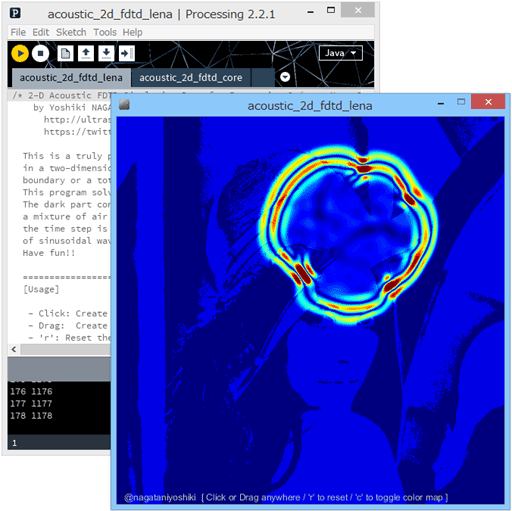
A sketch (program) of 2-D Acoustic FDTD for Processing 2 & 3. This sketch has been tested with Processing 2.2.1 and 3.1.2 (64bit) both on Windows and OSX. You can easily change the model by preparing your own image files. You can also change the acoustic properties (wave speed etc.) by changing the parameters in the source code directly. Please see the "Stability Conditions" section below.
Prior to running this sketch, please setup Processing 2 or 3. Then, open and run "acoustic_2d_fdtd_processing2.pde" or "acoustic_2d_fdtd_processing3.pde" file. No additional library is required.
- First vertion for Processing 2.x published on: Nov. 28th, 2014
- Version for Processing 3.0: Aug. 2nd, 2016
- CC-BY-SA 3.0 License is specified: Aug. 2nd, 2016

- MATLAB version (2-D Acoustic FDTD) [GitHub]
- 2-D Acoustic FDTD simulation with homogeneous media surrounded by total reflecting walls. (This is one of the simplest but the slowest program of the FDTD method.)
The sciprts using GPU device is also provided so that you can compare the speed of calculation between CPU and GPU.
- First vertion published on: Oct. 19th, 2016
- Speed Comparison among Various Languages (2-D Acoustic FDTD) [GitHub]
- 2-D Acoustic FDTD simulation in C (.c),Fortran 90 (.f90),Julia (.jl),MATLAB (.m),Processing 3 (.pde),Perl (.pl),Python 3 (.py),and Scilab (.sci) languages. Although the comments are written in Japanese, I am sure it is very easy to understand what is done in the programs.
- First vertion published on: Aug. 27th, 2018
The Overview of the Acoustic FDTD and the Elastic FDTD
- Stability Conditions of the FDTD method
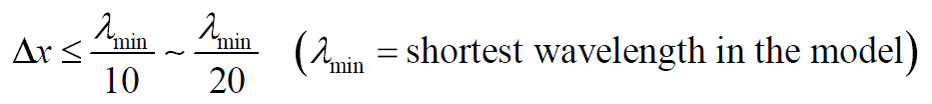
- For the stable and precise calculation of FDTD, the Δx [m] (spatial resolution) and Δt [s] (temporal resolution = time step) should satisfy the relationships below:
 , (1)
, (1)
 . (2)
. (2)
The condition (1) is empirically recommended for good precision of the calculation. In contrast, the condition (2), called Courant–Friedrichs–Lewy (CFL) condition, is strictly required for the stable simulation.
The wavelength λ [m] is calculated by
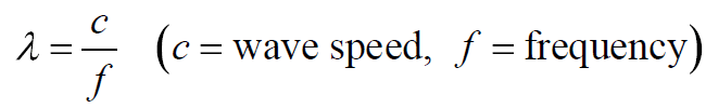 , (3)
, (3)
and the wave speed (longitudinal wave) c [m/s] in fluid media and solid media are calculated by the following equations, respectively:
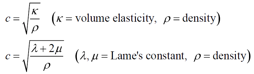 . (4)
. (4)
If you change the acoustic parameters and/or the frequency of the initial wave in the demo programs, please choose the values of Δx (dx) and Δt (dt) carefully to satisfy the conditions (1) and (2). - Acoustic FDTD
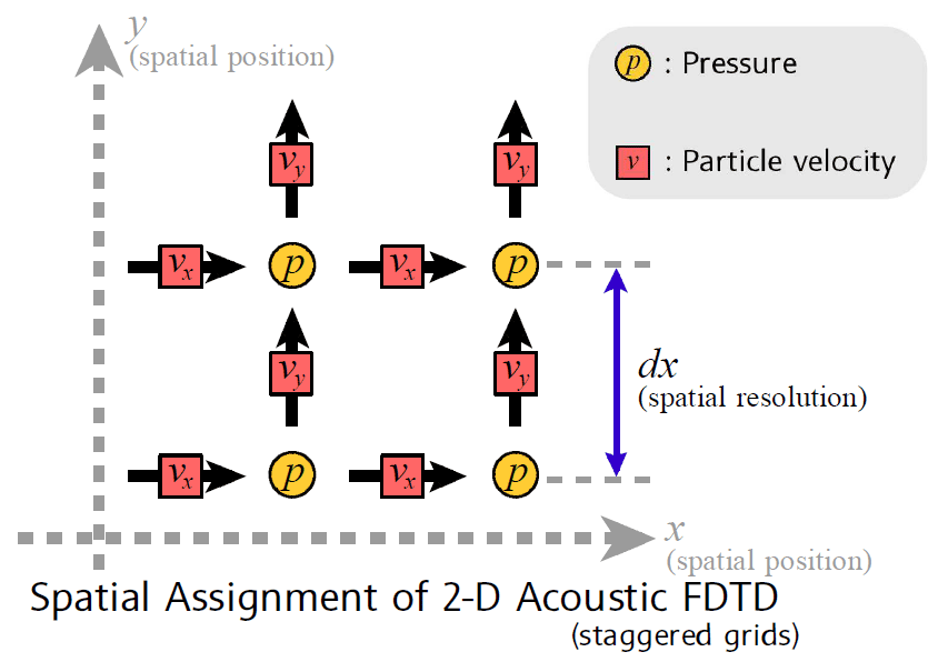
- The acoustic FDTD is a method for the calculation of the sound in fluid media (i.e. air or liquid).
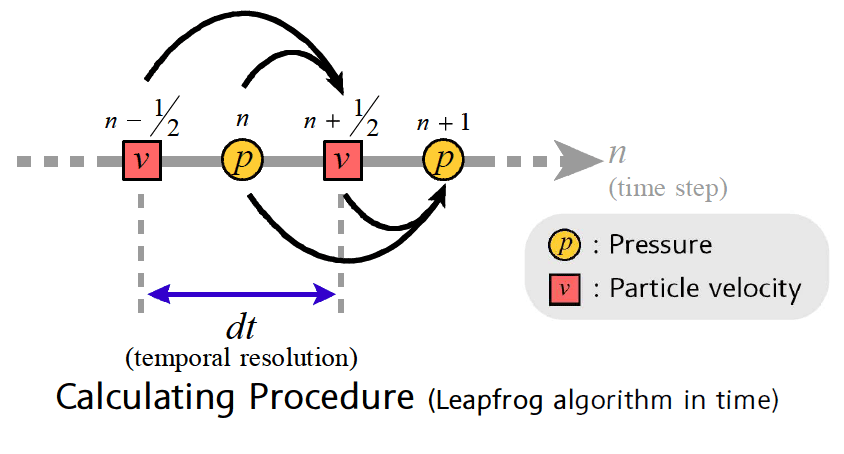
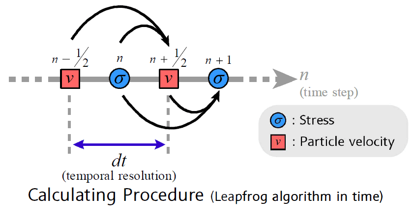
In the acoustic FDTD method, particle velocity and sound pressure (scalar value) in the simulation field are aligned alternately, which is called staggered grids. Then, pressure and particle velocity are updated alternately, which is called leapfrog algorithm. Thanks to this elegant design, the temporal evolution of the sound field in the model can be calculated step by step.
cf. The governing equations of the acoustic FDTD are:
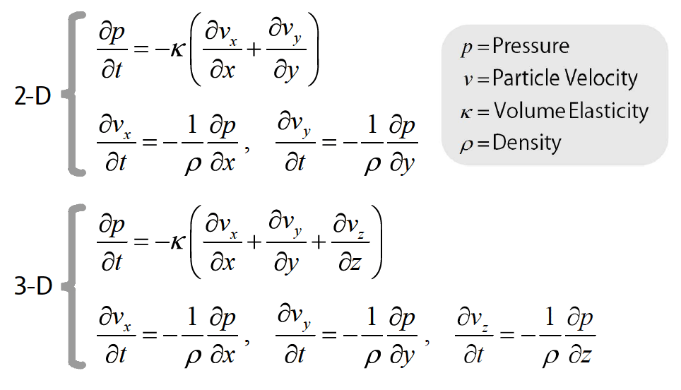 .
.
- Elastic FDTD
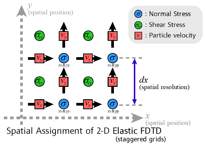
- The elastic FDTD is a method for the calculation of the sound in solid media, where shear waves can propagate as well as the longitudinal waves.
In the elastic FDTD method, particle velocity, normal stress, and shear stress (vector values) in the simulation field are aligned alternately. Then, stresses and particle velocity are updated alternately.
cf. The governing equations of the elastic FDTD are:
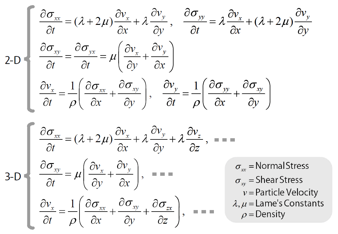 .
.
- シミュレーション結果の可視化手法 [in Japanese]
- 音波伝搬シミュレーションの計算結果の可視化手法 についての資料(PDF)を公開しています。
(技術情報協会から2018年に刊行予定の「遮音・吸音材料」の原稿として寄稿した内容を元にしています。)
Technique for the Visualization of the Results of FDTD method
Who am I ?
Yoshiki NAGATANI (Ph.D. (Engineering))
- Associate Professor at Kobe City College of Technology, Japan (Department of Electronics)
- Visiting Researcher, Université Paris-Est Créteil, France (UPEC)
![]() github.com/nagataniyoshiki/
github.com/nagataniyoshiki/
![]() @nagataniyoshiki
@nagataniyoshiki
![]() www.researchgate.net/profile/Yoshiki_Nagatani
www.researchgate.net/profile/Yoshiki_Nagatani
![]() www.linkedin.com/in/nagataniyoshiki
www.linkedin.com/in/nagataniyoshiki
![]()
![]()
[ Please see my website also: http://ultrasonics.jp/nagatani/e/ ]
Acknowledgement
I deeply appreciate Dr. Ryosuke TACHIBANA (![]() @ro_tachi) (The University of Tokyo) providing an insightful idea of creating visualized simulation projects and testing the programs.
@ro_tachi) (The University of Tokyo) providing an insightful idea of creating visualized simulation projects and testing the programs.